

linear,
sort of linear but magnetic interactions may be more influential than temperature..
linear,
sort of linear but magnetic interactions may be more influential than temperature..
There are limits to any mathematical model and a common beginner’s mistake is to extend their data beyond the limits of the defining data. Put another way: interpolation is forgiven but extrapolation is forbidden, especially when breaking new ground with new technology with still poorly understood mechanisms.

There are limits to any mathematical model and a common beginner’s mistake is to extend their data beyond the limits of the defining data. Put another way: interpolation is forgiven but extrapolation is forbidden, especially when breaking new ground with new technology with still poorly understood mechanisms.
Yes, any mathematical model is a caricature. But such models are useful aids to understanding. It is not a mistake to use them at the stage of investigation you find yourself in now.
The model I have been considering is much more general and the results are more robust than you believe. To be fair, I haven't talked much recently about the more general setting. I'll put something together on this subject. May take a couple of days.

Yes, any mathematical model is a caricature.
I note that the modeled LENR process is active at room temperature (20C in my model). Mizuno measured a value of Ea = 0.165 eV/K/atom for the Arrhenius activation energy.
Please note that Mizuno had a typo.... before you model anything..Bruce
there is no such thing as an Ea measured in 0.165 eV/K/atom
a caricature is one thing ....a typo is another,,
Here is a more generalized perspective on a simple model of the sort of system that Mizuno, Rothwell, Daniel_G and others claim to be dealing with.
The model consists of a thermal mass that can be heated either externally (i.e., by external command) or internally through some sort of LENR mechanism. The mass undergoes Newtonian cooling and the internal heating is said to depend in temperature with higher temperatures evoking greater heat production. That's it. That is the model. It is purposely kept simple
One can try and understand the behaviour of the model by setting up corresponding equations and then integrating them to find the time evolution of temperature. I have already done that in previous posts. But another way to think about the model is to identify equilibrium points (where temperature is stable) and keep track of their properties.
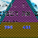
In the first diagram below, the 2 upper panels show the balance of heating (red) and cooling (blue) in the thermal mass in the null case where there is no internal heating. Power dissipated by Newtonian cooling depends linearly on the difference between the temperature of the thermal mass and ambient room temperature and so appears as a straight diagonal line. Power input into the system via external heating is treated as an control variable here and does not depend on temperature. It is thus a horizontal line in the plots. Points where the red and blue lines cross are equilibrium points where cooling just balances heating. The top left panel shows the equilibrium for a low value of external heating and the top right panel shows the equilibrium associated with a higher input. The equilibria are stable. In each case, if you bump the temperature down a little bit, heating rises above cooling to restore the temperature back to the equilibrium. If you bump the temperature up a little bit, cooling wins out over heating to again restore the equilibrium.
It can be seen that the temperature at which equilibrium is reached depends on the level of external heating inputted to the system. The bottom panel shows this dependence.
Now ... add internal (temperature-sensitive, LENR) heating to the mix. This is heat generation that is said to be small at low temperatures and higher at higher temperatures. This is shown In the figure below by a curved red line. Newtonian cooling is still in place and equilibria still occur at points where the red and blue lines cross. But this time, because of the general nature of the internally generated heating, 2 equilibria are present for any value of external heating. The lower-temperature equilibrium is stable to pertubations, just as in the previous case, but the higher-temperature equilibrium is unstable. If the system is at this upper equilibrium and temperature fluctuates down just a bit, cooling will slightly predominate over heating and the system will drift down away from the equilibrium point. Jostle the temperature just a little bit above the equilibrium and more internal heating turns on, driving the system up and up to eventual meltdown.
For this condition, you can envision external heating as driving the red heating curve vertically upward. An example is shown in the top right panel. There are still 2 equilibria, one stable and one unstable, but they are now closer together in temperature. Increasing external heating even more will drive the red curve even higher and you can see that eventually the 2 equilibria will coalesce and then disappear altogether. Once they have disappeared, you have reached an input level where no equilibrium is possible and the system escapes to meltdown.
The dependence of the equilibrium points on external heating is shown in the bottom panel. For many levels of external heating there are 2 equilibria, but past a threshold (called a bifurcation point) temperature escape occurs. The small arrows show the direction of temperature change at different points in the space.
So ... adding temperature-sensitive internal heating to the model qualitatively changes behaviour. And the point to make here is that the nature of the internal heating is not closely specified. You can have many different curves -- exponential, nonexponential, what have you -- and over a wide range of parameters this threshold behaviour will emerge. This is a behaviour I would look for in these systems as an indication that internal heating really is at work.
Power dissipated by Newtonian cooling depends linearly on the difference between the temperature of the thermal mass and ambient room temperature and so appears as a straight diagonal line
It's a nice start Bruce. But of course it's only valid for small temperature rise above ambient, and where conductive cooling is the dominant heat path. I suspect and hope you will extend this model to include more realistic non-linear behavior with both convective and radiative cooling considered.
Very deep, simple and enough realistic study Bruce__H .
Your model well explains if "Internal" xsh are generated, you have to stop the external heater to allow time for excess heat to escape then restart it, again and again following ON/OFF cycles.
These running cycles will allow to not exceed the equilibrium point you mentioned.
Never i have seen this behavior by experiments presented on the forum, i conclude never xsh were produced.
Display MoreHere is a more generalized perspective on a simple model of the sort of system that Mizuno, Rothwell, Daniel_G and others claim to be dealing with.
The model consists of a thermal mass that can be heated either externally (i.e., by external command) or internally through some sort of LENR mechanism. The mass undergoes Newtonian cooling and the internal heating is said to depend in temperature with higher temperatures evoking greater heat production. That's it. That is the model. It is purposely kept simple
One can try and understand the behaviour of the model by setting up corresponding equations and then integrating them to find the time evolution of temperature. I have already done that in previous posts. But another way to think about the model is to identify equilibrium points (where temperature is stable) and keep track of their properties.
In the first diagram below, the 2 upper panels show the balance of heating (red) and cooling (blue) in the thermal mass in the null case where there is no internal heating. Power dissipated by Newtonian cooling depends linearly on the difference between the temperature of the thermal mass and ambient room temperature and so appears as a straight diagonal line. Power input into the system via external heating is treated as an control variable here and does not depend on temperature. It is thus a horizontal line in the plots. Points where the red and blue lines cross are equilibrium points where cooling just balances heating. The top left panel shows the equilibrium for a low value of external heating and the top right panel shows the equilibrium associated with a higher input. The equilibria are stable. In each case, if you bump the temperature down a little bit, heating rises above cooling to restore the temperature back to the equilibrium. If you bump the temperature up a little bit, cooling wins out over heating to again restore the equilibrium.
It can be seen that the temperature at which equilibrium is reached depends on the level of external heating inputted to the system. The bottom panel shows this dependence.
Now ... add internal (temperature-sensitive, LENR) heating to the mix. This is heat generation that is said to be small at low temperatures and higher at higher temperatures. This is shown In the figure below by a curved red line. Newtonian cooling is still in place and equilibria still occur at points where the red and blue lines cross. But this time, because of the general nature of the internally generated heating, 2 equilibria are present for any value of external heating. The lower-temperature equilibrium is stable to pertubations, just as in the previous case, but the higher-temperature equilibrium is unstable. If the system is at this upper equilibrium and temperature fluctuates down just a bit, cooling will slightly predominate over heating and the system will drift down away from the equilibrium point. Jostle the temperature just a little bit above the equilibrium and more internal heating turns on, driving the system up and up to eventual meltdown.
For this condition, you can envision external heating as driving the red heating curve vertically upward. An example is shown in the top right panel. There are still 2 equilibria, one stable and one unstable, but they are now closer together in temperature. Increasing external heating even more will drive the red curve even higher and you can see that eventually the 2 equilibria will coalesce and then disappear altogether. Once they have disappeared, you have reached an input level where no equilibrium is possible and the system escapes to meltdown.
The dependence of the equilibrium points on external heating is shown in the bottom panel. For many levels of external heating there are 2 equilibria, but past a threshold (called a bifurcation point) temperature escape occurs. The small arrows show the direction of temperature change at different points in the space.
So ... adding temperature-sensitive internal heating to the model qualitatively changes behaviour. And the point to make here is that the nature of the internal heating is not closely specified. You can have many different curves -- exponential, nonexponential, what have you -- and over a wide range of parameters this threshold behaviour will emerge. This is a behaviour I would look for in these systems as an indication that internal heating really is at work.
If we need alternating ON-OFF cycles to elicit XSH at equilibrium, then why not power the system with sine-wave AC? Then XSH should be measurable in a continuum proportional to the amplitude of Ein, the energy applied into the system. And thus controllable by turning a rheostat up or down.
If we need alternating ON-OFF cycles to elicit XSH at equilibrium, then why not power the system with sine-wave AC?
I undertook a long series of experiments attempting to trigger LENR in some pretty reliable fuel mixes using AC solenoid heaters with zero success. The switch in magnetic field polarity is the problem I suspect. Intermittent DC with fast rise times seems to be much better as a triggering mechanism.

if "Internal" xsh are generated, you have to stop the external heater to allow time for excess heat to escape then restart it, again and again following ON/OFF cycles.
True. That is why Russ and I (at Russ's instigation) used heater control thermocouples in direct contact with the fuel-tube- only separation was around 1.5mm of fused alumina, which has excellent thermal conductivity. The entire system had very low thermal mass.

But of course it's only valid for small temperature rise above ambient, and where conductive cooling is the dominant heat path.
I don't really have a feel for the relative contributions of conductive vs radiative cooling in Daniel's system. He has calibrations (empty reactor with no nickel mesh) showing an almost linear dependence of steady state temperature on input power up to about 200C. So ... there little indication of radiative cooling playing a major role in that region. I believe he has calibrations to higher temperatures too but I haven't seen them.
。
校正用ヒーターについても同じことが言えます。
では、なぜキャリブレーションヒーターで過剰な熱を確認できないのでしょうか。
これを説明してください。
The same discussion can be made about heaters for calibration.
So why can't we see excess heat with the calibration heater?
Please explain this.
If we need alternating ON-OFF cycles to elicit XSH at equilibrium, then why not power the system with sine-wave AC?
I suppose that might be too fast. In the early days of cold fusion, Takahashi had good results from turning the power on and off, then on again. He called this the L-H (low-high) method. The period is several hours, not 60 Hz. See, for example:
https://www.lenr-canr.org/acrobat/TakahashiAanomalouse.pdf
Fleischmann strongly advocated a heat pulse. That is, turning up electrolysis to add a lot of heat rapidly. He used the pulse as a way to calibrate the cell, or to confirm there was excess heat. I showed some of his graphs and summarized this method here, pages 14 - 16:
https://www.lenr-canr.org/acrobat/Fleischmanlettersfroa.pdf
You can find out much more from his letters in this collection, and his papers.
He said that when the reaction was already started, the pulse can enhance it, as you see in these graphs. It is not clear whether it triggers a reaction in a sample that was not already producing low level heat. I think he said it does not.
I don't really have a feel for the relative contributions of conductive vs radiative cooling in Daniel's system. He has calibrations (empty reactor with no nickel mesh) showing an almost linear dependence of steady state temperature on input power up to about 200C. So ... there little indication of radiative cooling playing a major role in that region. I believe he has calibrations to higher temperatures too but I haven't seen them.
I agree with Magicsound that the relative contributions of conductive, convective and radiative cooling have a complex non-linear relationship over the range of temperatures involved. When you see linear dependence below 200C, I submit that our measurement methods do not fully resolve what is going on in this range and I don't care because the interesting part takes place at higher temperatures so this scenario is deliberate.
Its rather like someone measuring flatness of a bridge and then claiming the Earth is flat. When you can't resolve small changes this is the result you see.
Just because you don't see radiative effects below 200C, doesn't mean you don't need to model them at they are proportional to T°K^4.
I commend Bruce_H for his work but its very much like the climate modelers who can't model clouds and geothermal heat and then have to "fudge factor" in water vapor effects in an ill-fated attempt to make their models fit the real world data. Yes its a massive amount of work and computing power involved and it looks all high-tech and impressive but since you can fudge your way to any result you desire its totally meaningless.
Similarly, models for LENR/Cold-fusion are not possible with the low resolution data we have from current calorimeters. We have to push the metrology part in order to get sufficient data with low enough uncertainty before we sincerely get into modeling. Bruce_H may be ahead of the curve in his thought experiments on modeling, and who knows? Maybe he may find something that turns out to be useful in the future.
In the meantime, we focus our efforts on the ways to get better data and move practical CF technology forward.
As for pulsing, our best results so far were with giant thermal capacitors (thermal mass) done over long periods of time and this takes out a lot of noise and results in very clean and precise data at the cost of very long times required for each data point. I personally don't believe that short time resolution is the answer to anything. Current calorimeters just cannot resolve the heat accurately at short time scales. It's a direction not interesting for me personally.
 Display More
。
校正用ヒーターについても同じことが言えます。
では、なぜキャリブレーションヒーターで過剰な熱を確認できないのでしょうか。
これを説明してください。
The same discussion can be made about heaters for calibration.
So why can't we see excess heat with the calibration heater?
Please explain this.
I am not so sure we could explain the excess heat, but we would like to prove it.
If a calibration did show excess heat, for example, what is the procedure to deal with the results?
Current calorimeters just cannot resolve the heat accurately at short time scales. It's a direction not interesting for me personally.
The D-system by Takahashi et al seems to be very responsive...
@ Alan Smith - yes, of course you are correct - long timescales between DC pulses are the way to go - although Brillouin Energy use the 'skin effect' with rapid DC switching in their HHT's. They follow presumably the Widon-Larson model where electrons 'bunch' on the surface of the cathode to catalyse LENR fusion. But it could also be due to transient formation of ultra-dense hydrogen formation at active NAE's ie cracks in the surface of the cathodes they use. There does not appear to be one unifying theory behind LENR, so it is very difficult to decide on which theory is the truth.
The D-system by Takahashi et al seems to be very responsive...
His lab is stable for 4 digits after the decimal point. So he gets changes of +/- 0.0001C ! This is always relative to the calibration!