Bruce__H Member
  • Member since Jul 22nd 2017
  • Last Activity:

Posts by Bruce__H

    This fuel was just one sample we used for 1 day (unluckily I did head home the next day..). So we have about 20 spectra.

    How important it was we noticed months later....

    Thank you for your answer.


    How many of the 20 spectra were used to generate the specific findings you report in your manuscript?


    It is said so...Taken at 380C...


    I had in mind that you may have taken several samples at 380C.


    I am trying to understand your manuscript. You will encounter the same type of questions from anyone trying to seriously understand it because some things are not clearly stated.


    What about the rest of the results in the manuscript, how many separate spectral samples were used to generate your results?

    As said you never did measure a spectrum or a background. It is never random....

    This is a technical feature of radioactive decay that you appear not to understand. I am surprised. Please ask your friends on this point, or consult a textbook.


    While the average rate of radioactive decay is a stable physical property of nuclei, the actual timing of decay events is a random process. One therefore expects the arrival of events to be a Poisson process and, for low event counts (of the type you show), Poisson noise will be dominant. This noise, however, becomes a smaller and smaller part of the signal as the counts in each bin increase. That is why long-duration samples are desirable -- they increase the bin counts and so reduce the relative impact of Poisson noise. If you are prevented from taking long-duration samples because your conditions are not stationary, then averaging of noncontiguous samples to reduce Poisson noise is appropriate, as THHuxelyNew pointed out.

    Once more this is a delta spectrum modified by the Theremino parameters for nearby bucket contributions.


    A real spectrum is a set of histogram values. In the tables I form the deltas from the buckets.

    Thank you for your answer. I find, however, that it does not clear up my confusion.


    I mentioned in a previous post (here) that the 2 spectra in your Figure 1 (derived from activity at 2 different temperatures) are too similar. They are so similar that they cannot be simply showing background-subtractd event counts, as you claim. Instead, I think that these are somehow showing averaged counts. If these were straightforward event counts, the probabilistic nature of radioactive decay means that the standard deviation around each bin count would be equal to the square root of the bin count itself. Instead the 2 spectra you show in Figure 1 ) differ only by fractions of a standard deviation at most energy levels. Modifications "... by the Theremino parameters for nearby bucket contributions" would not explain this near similarity between spectra from completely different samples.


    From experimenting with the Theremino software, I believe that the spectra you are showing in Figures 1 and 2 of your ResearchGate manuscript were gathered while a "progressive integration" algorithm was engaged (i.e., the "iIntegr. time" button was pressed. Is this so? If this algorithm is engaged while data are being taken, the values in both the data histograms and the screen image are not event counts.

    Did you have the "Integr. time" button in the Theremino control dialog box pressed when you took the data for Figures 1 and 2?

    Wyttenbach

    I see that in response to my question you have inserted a laughing face icon.

    Does this mean that you intend not to answer my question?


    Figures 1 and 2 of your ResearchGate manuscript definitely do not show event counts along their vertical axes. If these really were counts, the Poisson noise would be a much larger contribution to the spectra than is seen. I would like to find out what is being portrayed here. Please take this opportunity to answer reasonably.

    What do you think about the sentence in the text? Counts above background....?

    In the text, you never specifically refer to the vertical axis visible in Figures 1 and 2.


    Did you have the "Integr. time" button in the Theremino control dialog box pressed when you took the data for Figures 1 and 2?

    Wyttenbach

    What do the numbers on the vertical axis mean in the spectra in Figures 1 and 2? Here, for instance, is Figure 1....


    I had initially thought that the numbers were event counts (over your 10-minute sampling time) but, as I explained earlier, the lack of Poisson noise indicates that this is not so. Now having looked at the Theremino software and its documentation I think that you must have had the "Integr. time" button pressed while you took the spectra. If this is true then the numbers do not represent actual counts. Instead, they represent quantities calculated from some sort of averaging procedure that is engaged when the "Integr. time" button is pressed.


    Do you know what the numbers mean?

    Cosmic Rays. You would be surprised what they can do and how often you might see them

    Fair enough. As a feature that might occur during active runs but is extrinsic, shouldn't this be regarded as a a background feature? Why try to exclude them from the background?

    If you do short measurement runs then these are prone to background peeks. Better you know them!

    I don't understand how this responds to any f the observations I just made. Nor do I understand how it fits with anything you have said earlier.


    I'm not even sure what you mean here by a background peak. Can you point out for me what you regard as a background peak in your Figure 2?

    Exactly this - averaging background - is not serious science. We here did used two different backgrounds (space angles) without and without experiment and we always use the maximum of both to discriminate a signal. Averaging gives you many more signals albeit some of them can be artifacts = random peaks.

    Background averaging is just fine if done properly. The random peaks you mention are exactly the sort of thing that averaging should reduce.


    There is something about how you are taking and processing your backgrounds and your other spectra that just isn't making sense. I think that there is something about your procedure you haven't explained and that is why people aren't understanding what you are saying.


    In particular, I don't understand the relationship between your backgrounds and the active fuel in your setup. Why do you say ... "long run backgrounds cannot be use to discriminate lines as possible bursts are hidden"? What bursts? Bursts of what?

    A fourier analysis without any previous algorithmic filtering of the data would resolve this discrepancy. We have used FFT in biophysics to study single-channel voltage fluctuations in the past on an old state of the art (at that time (1980) PDP-11 computer system.

    Frequency-domain analysis of single-channel patch-clamp data in 1980? That would be right at the forefront of physiological research back then. Respect!

    10keV = 17 bins and a peek displayed as such in a spectrum spawn at least three bins because the software does so. You just waste time with an interpolated curve that hides the reality...

    I give detailed peek counts in the table including background....

    The problem is that the data shown in your tables does not allow readers to see how much variation exists between successive spectra.


    Figures 1 and 2 need to be redone anyway -- because they are blurry screen captures with unreadable labels -- so why not replot these figures using data straight from the output of the MCA? Or post the raw data and let people plot them for themselves.

    A gamma spectrum has nothing to do with noise. Only a part of background is real noise... A calibration source typically has some 1000bq.

    A calibration source is 1000bq but your detector is seeing nothing like this rate of gamma events. The bin counts you report are only on the order of 0-40 counts per 10 minutes and are thus susceptible to Poisson noise.


    For the low number of counts you report, Poisson noise is a major factor in the signal. If the counts were higher, the impact of this type of noise would be much smaller. The signal-to-noise ratio for Poisson noise = sqrt(n) where n is the bin count. In other words, the signal-to-noise ratio improves as the square root of the number of counts per bin. See https://radio.astro.gla.ac.uk/old_OA_course/pw/qf3.pdf

    Typical beginners error. A stable physical process delivers a stable gamma count. Why do you believe we can measure half lives??

    We differ on the most fundamental issues of the physics here.


    The radioactive decay processes I know about are probabilistic. To answer your question ... I believe we can measure half-lives as bulk phenomena, but on a microscopic scale the probabilistic nature of the process results in Poisson noise as I outlined.


    Thorium 234 has a half life of 24 days. Suppose you have 2 atoms of Thorium 234 sitting in a box. Are you somehow arguing that those 2 atoms will sit there until 24 days are up and then one of them will decay? That is where you seem to be heading.

    I continue to try and understand some of the results presented by Wyttenbach in his most recent ResearchGate posting (A new experimental path to nucleosynthesis)


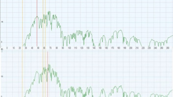
    I have had trouble understanding the nature of the gamma spectra displayed in this work. In particular, in thinking about things, I don't understand why the noise in some spectra seems so low. Figure 1, for instance, shows background-subtracted spectra at 250C (top, below) and 380C (bottom, below). Both spectra are taken over 10 minutes.


    What we see here is a remarkable similarity between the 2 spectra. They are not identical -- after all they are taken at different times and different temperatures -- but for the most part the bumps and valleys in the top spectrum also occur in the bottom one. The similarity does not just consist in the 2 spectra showing mainly the same peaks (which is OK), but in the peaks being the same height n both spectra. Indeed, if you superimpose these traces they fit over top of each other very closely at many many points.


    My puzzlement here is that the event count in each bin of a spectrum should be roughly Poisson distributed (due to the random timing of gamma events). Following from this, the standard deviation of counts in each bin should be about the square root of the count number itself. Thus if we were to acquire the same spectrum again (over a similar interval) the count number in each bin should differ slightly from the first values. And, if we acquired and reacquired the same spectrum over and over, we should find that the count in any bin should vary with the square root of the mean count as just noted.


    Now, look at the red vertical line in the top spectrum (at about 49 keV). It happens to lie near the peak of a feature that is also present in the lower spectrum. In the top spectrum, the bin count at 49 keV is (estimating by eye) 19. In the bottom spectrum the bin count is about 18. These count values are close. Too close by my reckoning! I calculate that the standard deviation of counts at this energy should be about 5.5 (because total counts at this energy [background + signal] is 30 counts and the square root of 30 is about 5.5). In light of this, the 1-count difference between the upper and lower spectra at this energy is statistically unlikely.


    You can repeat this observation for any energy shown in Figure 1 and get the same result. The difference between the 2 spectra at most energies is many times smaller than expected. So this is not just a statistical fluke that happens to occur at 49 keV. It is at all energies. And I don't understand why this is. Wyttenbach says a (undescribed) smoothing algorithm has been used before displaying the spectra, but it is not immediately apparent to me how this could account for such a radical reduction in variation between them.


    Does anyone know what might be going on?

    The spikes are lines that sometimes match and sometimes due to algorithm are slightly displaced. So as said either you have the data and can interpret it or you don't. Everybody that joins research will have access to data. But this needs some credibility, time and money and some valuable experience.

    You are the one who posted these data. You now need to explain them in a way that others can understand. No one here understands what you have done.

    The long spectrum was one of the first done by Russ and is from a highly productive reaction. So in fact it is the fist one from a cold fusion reaction. ...

    I'm not sure where you are heading here. Are you saying that you currently do not interpret the spike-like features as spectrographic peaks?

    magicsound

    I follow most of what you say. But when I said that the spikey things don't seem to be noise what I meant is that I think Wyttenbach is interpreting them as genuine spectroscopic peaks.


    The data are said to have been gathered over the course of more that 3 hours. I know it is very tough to see the vertical scale on the depicted spectrum ... but full scale is almost 5000 counts. Most of the peaks rise 1000 counts or so above their neighbouring valleys. This all seems to be beyond the realm of stochastic effects you mention.


    Also, Wyttenbach displays the following background taken in the same lab with (I think, but am not sure) the same equipment. It is said to be from a far shorter sample (10 minutes, vertical full scale is 26 counts). I don't see much noise here.


    Just a note. Of those 3 highlighted in red neutron waves the rightmost two do not exist (eyeballing). They are right down in the noise. I'd like to see a Bayesian analysis of the evidence for neutron waves at those values (rather than some other value). The evidence for hypothesised neutron waves from that graph would appear non-existent: and I would always defer to proper data analysis that would have to be Bayesian choosing hypotheses carefully.

    All those spikey things don't seem to be traditional noise. This is a 3-hour spectrum (according to Wyttenbach) and I think that the shot noise is low here compared with the signal. Instead, there is this forest of spikes, a few of which Wyttenbach puts forward as proof of his theories.


    My problem here is that there are so many features in the spectrum that almost any theory would seem to find support. Indeed, I have a theory! And here are 5 energy levels (in keV) that I predict should feature in the spectrum ... 105, 141, 169, 197, 238. I think I see them all. Does that mean my theory is right?